5 Understanding Data
Last edited: July 2023
Suggested Citation
Liao, Y. Understanding Data. In Bailey, P. and Zhang, T. (eds.), Analyzing NCES Data Using EdSurvey: A User’s Guide.
Once data are successfully read in (see how EdSurvey supports reading-in data for each study in Chapter 4), users can use the commands in the following sections to understand the data.
To follow along in this chapter, load the NAEP Primer dataset M36NT2PM and assign it the name sdf with the following call:
sdf <- readNAEP(path = system.file("extdata/data", "M36NT2PM.dat", package = "NAEPprimer"))5.1 Searching Variables
The colnames() function will list all variable names in the data:
colnames(x = sdf)
#>   [1] "ROWID"   "year"    "cohort"  "scrpsu"  "dsex"
#>   [6] "iep"     "lep"     "ell3"    "sdracem" "pared"
#>  [11] "b003501" "b003601" "b013801" "b017001" "b017101"
#>  [16] "b018101" "b018201" "b017451" "m815401" "m815501"
#>  [21] "m815601" "m815801" "m815701" "rptsamp" "repgrp1"
#>  [26] "repgrp2" "jkunit"  "origwt"  "srwt01"  "srwt02"
#>  [31] "srwt03"  "srwt04"  "srwt05"  "srwt06"  "srwt07"
#>  [36] "srwt08"  "srwt09"  "srwt10"  "srwt11"  "srwt12"
#>  [41] "srwt13"  "srwt14"  "srwt15"  "srwt16"  "srwt17"
#>  [46] "srwt18"  "srwt19"  "srwt20"  "srwt21"  "srwt22"
#>  [51] "srwt23"  "srwt24"  "srwt25"  "srwt26"  "srwt27"
#>  [56] "srwt28"  "srwt29"  "srwt30"  "srwt31"  "srwt32"
#>  [61] "srwt33"  "srwt34"  "srwt35"  "srwt36"  "srwt37"
#>  [66] "srwt38"  "srwt39"  "srwt40"  "srwt41"  "srwt42"
#>  [71] "srwt43"  "srwt44"  "srwt45"  "srwt46"  "srwt47"
#>  [76] "srwt48"  "srwt49"  "srwt50"  "srwt51"  "srwt52"
#>  [81] "srwt53"  "srwt54"  "srwt55"  "srwt56"  "srwt57"
#>  [86] "srwt58"  "srwt59"  "srwt60"  "srwt61"  "srwt62"
#>  [91] "smsrswt" "mrps11"  "mrps12"  "mrps13"  "mrps14"
#>  [96] "mrps15"  "mrps21"  "mrps22"  "mrps23"  "mrps24"
#> [101] "mrps25"  "mrps31"  "mrps32"  "mrps33"  "mrps34"
#> [106] "mrps35"  "mrps41"  "mrps42"  "mrps43"  "mrps44"
#> [111] "mrps45"  "mrps51"  "mrps52"  "mrps53"  "mrps54"
#> [116] "mrps55"  "mrpcm1"  "mrpcm2"  "mrpcm3"  "mrpcm4"
#> [121] "mrpcm5"  "m075201" "m075401" "m075601" "m019901"
#> [126] "m066201" "m047301" "m046201" "m066401" "m020101"
#> [131] "m067401" "m086101" "m047701" "m067301" "m048001"
#> [136] "m093701" "m086001" "m051901" "m076001" "m046001"
#> [141] "m046101" "m067701" "m046701" "m046901" "m047201"
#> [146] "m046601" "m046801" "m067801" "m066601" "m067201"
#> [151] "m068003" "m068005" "m068008" "m068007" "m068006"
#> [156] "m093601" "m053001" "m047801" "m086301" "m085701"
#> [161] "m085901" "m085601" "m085501" "m085801" "m019701"
#> [166] "m020001" "m046301" "m047001" "m046501" "m066501"
#> [171] "m047101" "m066301" "m067901" "m019601" "m051501"
#> [176] "m047901" "m053101" "m143601" "m143701" "m143801"
#> [181] "m143901" "m144001" "m144101" "m144201" "m144301"
#> [186] "m144401" "m144501" "m144601" "m144701" "m144801"
#> [191] "m144901" "m145001" "m145101" "m013431" "m0757cl"
#> [196] "m013131" "m091701" "m072801" "m091501" "m091601"
#> [201] "m073501" "m052401" "m075301" "m072901" "m013631"
#> [206] "m075801" "m013731" "m013531" "m051801" "m093401"
#> [211] "m093801" "m142001" "m142101" "m142201" "m142301"
#> [216] "m142401" "m142501" "m142601" "m142701" "m142801"
#> [221] "m142901" "m143001" "m143101" "m143201" "m143301"
#> [226] "m143401" "m143501" "m105601" "m105801" "m105901"
#> [231] "m106001" "m106101" "m106201" "m106301" "m106401"
#> [236] "m106501" "m106601" "m106701" "m106801" "m106901"
#> [241] "m107001" "m107101" "m107201" "m107401" "m107501"
#> [246] "m107601" "m109801" "m110001" "m110101" "m110201"
#> [251] "m110301" "m110401" "m110501" "m110601" "m110701"
#> [256] "m110801" "m110901" "m111001" "m111201" "m111301"
#> [261] "m111401" "m111501" "m111601" "m111801" "yrsexp"
#> [266] "yrsmath" "t089401" "t088001" "t090801" "t090802"
#> [271] "t090803" "t090804" "t090805" "t090806" "t087501"
#> [276] "t088301" "t088401" "t088501" "t088602" "t088603"
#> [281] "t088801" "t088803" "t088804" "t088805" "t091502"
#> [286] "t091503" "t091504" "c052801" "c052802" "c052804"
#> [291] "c052805" "c052806" "c052807" "c052808" "c052701"
#> [296] "c046501" "c044006" "c044007" "c052901" "c053001"
#> [301] "c053101" "sscrpsu" "c052601"
To conduct a more powerful search of NAEP data variables, use the searchSDF() function, which returns variable names and labels from an edsurvey.data.frame based on a character string. The user can specify which data source (either “student” or “school”) to search. For example, the following call to searchSDF() searches for the character string "book" in an edsurvey.data.frame and specifies the fileFormat to search the student data file:
searchSDF(string = "book", data = sdf, fileFormat = "student")
#>   variableName                                       Labels
#> 1      b013801                                Books in home
#> 2      t088804 Computer activities: Use a gradebook program
#> 3      t091503     G8Math:How often use Geometry sketchbook
#>   fileFormat
#> 1    Student
#> 2    Student
#> 3    Student
The levels and labels for each variable searched via searchSDF() also can be returned by setting levels = TRUE:
searchSDF(string = "book", data = sdf, fileFormat = "student", levels = TRUE)
#> Variable: b013801
#> Label: Books in home
#> Levels (Lowest level first):
#>      1. 0-10
#>      2. 11-25
#>      3. 26-100
#>      4. >100
#>      8. Omitted
#>      0. Multiple
#> Variable: t088804
#> Label: Computer activities: Use a gradebook program
#> Levels (Lowest level first):
#>      1. Never or hardly ever
#>      2. Once or twice/month
#>      3. Once or twice a week
#>      4. Almost every day
#>      8. Omitted
#>      0. Multiple
#> Variable: t091503
#> Label: G8Math:How often use Geometry sketchbook
#> Levels (Lowest level first):
#>      1. Never or hardly ever
#>      2. Once or twice/month
#>      3. Once or twice a week
#>      4. Almost every day
#>      8. Omitted
#>      0. Multiple
The | (OR) operator will search several strings simultaneously:
searchSDF(string="book|home|value", data=sdf)
#>    variableName
#> 1       b013801
#> 2       b017001
#> 3       b017101
#> 4       b018201
#> 5       b017451
#> 6       m086101
#> 7       m020001
#> 8       m143601
#> 9       m142301
#> 10      t088804
#> 11      t088805
#> 12      t091503
#>                                               Labels
#> 1                                      Books in home
#> 2                                  Newspaper in home
#> 3                                   Computer at home
#> 4         Language other than English spoken in home
#> 5                         Talk about studies at home
#> 6                              Read value from graph
#> 7  Apply place value                            (R1)
#> 8                       Solve for x given value of n
#> 9                               Identify place value
#> 10      Computer activities: Use a gradebook program
#> 11  Computer activities: Post homework,schedule info
#> 12          G8Math:How often use Geometry sketchbook
#>    fileFormat
#> 1     Student
#> 2     Student
#> 3     Student
#> 4     Student
#> 5     Student
#> 6     Student
#> 7     Student
#> 8     Student
#> 9     Student
#> 10    Student
#> 11    Student
#> 12    Student
A vector of strings will search for variables that contain multiple strings, such as both “book” and “home”; each string is present in the variable label and can be used to filter the results:
searchSDF(string=c("book","home"), data=sdf)
#>   variableName        Labels fileFormat
#> 1      b013801 Books in home    Student
To dive into a particular variable, use levelsSDF(). It returns the levels, the corresponding sample size, and label of each level.
levelsSDF(varnames = "b017451", data = sdf)
#> Levels for Variable 'b017451' (Lowest level first):
#>     1. Never or hardly ever (n = 3837)
#>     2. Once every few weeks (n = 3147)
#>     3. About once a week (n = 2853)
#>     4. 2 or 3 times a week (n = 3362)
#>     5. Every day (n = 3132)
#>     8. Omitted* (n = 575)
#>     0. Multiple* (n = 9)
#>     NOTE: * indicates an omitted level.
5.2 Displaying Basic Information
Some basic functions that work on a data.frame, such as dim, nrow, and ncol, also work on an edsurvey.data.frame. They help check the dimensions of sdf.
Basic information about plausible values and weights in an edsurvey.data.frame can be seen in the print function. The variables associated with plausible values and weights can be seen from the showPlausibleValues and showWeights functions, respectively, when setting the verbose argument to TRUE:
showPlausibleValues(data = sdf, verbose = TRUE)
#> There are 6 subject scale(s) or subscale(s) in this
#>   edsurvey.data.frame:
#> 'num_oper' subject scale or subscale with 5 plausible
#>   values.
#>   The plausible value variables are: 'mrps11',
#>   'mrps12', 'mrps13', 'mrps14', and 'mrps15'
#>
#> 'measurement' subject scale or subscale with 5
#>   plausible values.
#>   The plausible value variables are: 'mrps21',
#>   'mrps22', 'mrps23', 'mrps24', and 'mrps25'
#>
#> 'geometry' subject scale or subscale with 5 plausible
#>   values.
#>   The plausible value variables are: 'mrps31',
#>   'mrps32', 'mrps33', 'mrps34', and 'mrps35'
#>
#> 'data_anal_prob' subject scale or subscale with 5
#>   plausible values.
#>   The plausible value variables are: 'mrps41',
#>   'mrps42', 'mrps43', 'mrps44', and 'mrps45'
#>
#> 'algebra' subject scale or subscale with 5 plausible
#>   values.
#>   The plausible value variables are: 'mrps51',
#>   'mrps52', 'mrps53', 'mrps54', and 'mrps55'
#>
#> 'composite' subject scale or subscale with 5
#>   plausible values (the default).
#>   The plausible value variables are: 'mrpcm1',
#>   'mrpcm2', 'mrpcm3', 'mrpcm4', and 'mrpcm5'
showWeights(data = sdf, verbose = TRUE)
#> There is 1 full sample weight in this
#>   edsurvey.data.frame:
#>   'origwt' with 62 JK replicate weights (the
#>   default).
#>     Jackknife replicate weight variables associated
#>     with the full sample weight 'origwt':
#>     'srwt01', 'srwt02', 'srwt03', 'srwt04', 'srwt05',
#>     'srwt06', 'srwt07', 'srwt08', 'srwt09', 'srwt10',
#>     'srwt11', 'srwt12', 'srwt13', 'srwt14', 'srwt15',
#>     'srwt16', 'srwt17', 'srwt18', 'srwt19', 'srwt20',
#>     'srwt21', 'srwt22', 'srwt23', 'srwt24', 'srwt25',
#>     'srwt26', 'srwt27', 'srwt28', 'srwt29', 'srwt30',
#>     'srwt31', 'srwt32', 'srwt33', 'srwt34', 'srwt35',
#>     'srwt36', 'srwt37', 'srwt38', 'srwt39', 'srwt40',
#>     'srwt41', 'srwt42', 'srwt43', 'srwt44', 'srwt45',
#>     'srwt46', 'srwt47', 'srwt48', 'srwt49', 'srwt50',
#>     'srwt51', 'srwt52', 'srwt53', 'srwt54', 'srwt55',
#>     'srwt56', 'srwt57', 'srwt58', 'srwt59', 'srwt60',
#>     'srwt61', and 'srwt62'
The functions getStratumVar and getPSUVar return the default stratum variable name or a PSU variable associated with a weight variable.
getStratumVar(data = sdf, weightVar = "origwt")
#>   stratum
#> "repgrp1"
getPSUVar(data = sdf, weightVar = "origwt")
#>      psu
#> "jkunit"
5.3 Keeping or Removing Omitted Levels
EdSurvey uses listwise deletion to remove special values in all analyses by default. For example, in the NAEP Primer data, the omitted levels are returned when print(sdf) is called: Omitted Levels: 'Multiple', 'NA', 'Omitted'. By default, these levels are excluded via listwise deletion in EdSurvey analytical functions. To use a different method, such as pairwise deletion, set defaultConditions = FALSE when running your analysis.
5.4 Exploring Data
This section introduces three basic R functions (both EdSurvey and non-EdSurvey) commonly used in the data exploration step, as follows:
summary2()produces both weighted and unweighted descriptive statistics for a variable.edsurveyTable()produces cross-tabulation statistics.ggplot2produces a variety of exploratory data analysis (EDA) plots.
5.4.1 summary2()
summary2() takes the following four arguments in order:
-
data: AnEdSurveyobject. -
variable: Name of the variable you want to produce statistics on. -
weightVar: name of the weight variable orNULLif users want to produce unweighted statistics. -
dropOmittedLevels: IfTRUE, the function will remove omitted levels for the specified variable before producing descriptive statistics. IfFALSE, the function will include omitted levels in the output statistics.
The summary2 function produces both weighted and unweighted descriptive statistics for a variable. This functionality is quite useful for gathering response information for survey variables when conducting data exploration. For NAEP data and other datasets that have a default weight variable, summary2 produces weighted statistics by default. If the specified variable is a set of plausible values, and the weightVar option is non-NULL, summary2 statistics account for both plausible values pooling and weighting.
summary2(data = sdf, variable = "composite")
#> Estimates are weighted using the weight variable 'origwt'
#>    Variable     N Weighted N   Min.  1st Qu.   Median
#> 1 composite 16915   16932.46 126.11 251.9626 277.4784
#>       Mean  3rd Qu.    Max.      SD NA's Zero weights
#> 1 275.8892 301.1827 404.184 36.5713    0            0
By specifying weightVar = NULL, the function prints out unweighted descriptive statistics for the selected variable or plausible values:
summary2(data = sdf, variable = "composite", weightVar = NULL)
#> Estimates are not weighted.
#>   Variable     N   Min.  1st Qu. Median     Mean  3rd Qu.
#> 1   mrpcm1 16915 130.53 252.0600 277.33 275.8606 300.7200
#> 2   mrpcm2 16915 124.16 252.2100 277.33 275.6399 300.6900
#> 3   mrpcm3 16915 115.09 252.0017 277.19 275.6570 300.5600
#> 4   mrpcm4 16915 137.19 252.4717 277.44 275.7451 300.5767
#> 5   mrpcm5 16915 123.58 252.4900 277.16 275.6965 300.5000
#>     Max.       SD NA's
#> 1 410.80 35.89864    0
#> 2 408.58 36.08483    0
#> 3 398.17 36.09278    0
#> 4 407.41 35.91078    0
#> 5 395.96 36.10905    0
For a categorical variable, the summary2 function returns the weighted number of cases, the weighted percentage, and the weighted standard error (SE). For example, the variable b017451 (frequency of students talking about studies at home) returns the following output:
summary2(data = sdf, variable = "b017451")
#> Estimates are weighted using the weight variable 'origwt'
#>                b017451    N Weighted N Weighted Percent
#> 1 Never or hardly ever 3837  3952.4529      23.34245648
#> 2 Once every few weeks 3147  3190.8945      18.84483329
#> 3    About once a week 2853  2937.7148      17.34960077
#> 4  2 or 3 times a week 3362  3425.8950      20.23270282
#> 5            Every day 3132  3223.8074      19.03921080
#> 6              Omitted  575   194.3312       1.14768416
#> 7             Multiple    9     7.3676       0.04351168
#>   Weighted Percent SE
#> 1           0.4318975
#> 2           0.3740648
#> 3           0.3414566
#> 4           0.3156289
#> 5           0.4442216
#> 6           0.1272462
#> 7           0.0191187
By default, the summary2 function includes omitted levels; to remove those levels, set dropOmittedLevels = TRUE:
summary2(data = sdf, variable = "b017451", dropOmittedLevels = TRUE)
#> Estimates are weighted using the weight variable 'origwt'
#>                b017451    N Weighted N Weighted Percent
#> 1 Never or hardly ever 3837   3952.453         23.62386
#> 2 Once every few weeks 3147   3190.894         19.07202
#> 3    About once a week 2853   2937.715         17.55876
#> 4  2 or 3 times a week 3362   3425.895         20.47662
#> 5            Every day 3132   3223.807         19.26874
#>   Weighted Percent SE
#> 1           0.4367548
#> 2           0.3749868
#> 3           0.3486008
#> 4           0.3196719
#> 5           0.4467063
5.4.2 edsurveyTable()
edsurveyTable() creates a summary table of outcome and categorical variables. The three important arguments are as follows:
-
formula: Typically written asa ~ b + c, with the following meanings:-
ais a continuous variable (optional) for which the function will return the weighted mean. -
bandcare categorical variables for which the function will run cross-tabulations; multiple crosstab categorical variables can be separated using+symbol.
-
-
data: AnEdSurveyobject. -
pctAggregationLevel: A numeric value (i.e., 0, 1, 2) that indicates the level of aggregation in the cross-tabulation result’s percentage column.
The following call uses edsurveyTable() to create a summary table of NAEP composite mathematics performance scale scores (composite) of 8th-grade students by two student factors:
- dsex: gender
- b017451: frequency of talk about studies at home
pctAggregationLevel is by default set to NULL (or 1). That is, the PCT column adds up to 100 within each level of the first categorical variable dsex.
es1 <- edsurveyTable(formula = composite ~ dsex + b017451, data = sdf, pctAggregationLevel = NULL)| dsex | b017451 | N | WTD_N | PCT | SE(PCT) | MEAN | SE(MEAN) |
|---|---|---|---|---|---|---|---|
| Male | Never or hardly ever | 2350 | 2434.844 | 29.00978 | 0.6959418 | 270.8243 | 1.057078 |
| Male | Once every few weeks | 1603 | 1638.745 | 19.52472 | 0.5020657 | 275.0807 | 1.305922 |
| Male | About once a week | 1384 | 1423.312 | 16.95795 | 0.5057265 | 281.5612 | 1.409587 |
| Male | 2 or 3 times a week | 1535 | 1563.393 | 18.62694 | 0.4811497 | 284.9066 | 1.546072 |
| Male | Every day | 1291 | 1332.890 | 15.88062 | 0.5872731 | 277.2597 | 1.795784 |
| Female | Never or hardly ever | 1487 | 1517.609 | 18.20203 | 0.5078805 | 266.7897 | 1.519020 |
| Female | Once every few weeks | 1544 | 1552.149 | 18.61630 | 0.4892491 | 271.2255 | 1.205528 |
| Female | About once a week | 1469 | 1514.403 | 18.16358 | 0.5782966 | 278.7502 | 1.719778 |
| Female | 2 or 3 times a week | 1827 | 1862.502 | 22.33864 | 0.4844840 | 282.7765 | 1.404107 |
| Female | Every day | 1841 | 1890.918 | 22.67945 | 0.6553039 | 275.4628 | 1.219439 |
By specifying pctAggregationLevel = 0, such as in the following call, the PCT column adds up to 100 across the entire sample.
es2 <- edsurveyTable(formula = composite ~ dsex + b017451, data = sdf, pctAggregationLevel = 0)| dsex | b017451 | N | WTD_N | PCT | SE(PCT) | MEAN | SE(MEAN) |
|---|---|---|---|---|---|---|---|
| Male | Never or hardly ever | 2350 | 2434.844 | 14.553095 | 0.3738531 | 270.8243 | 1.057078 |
| Male | Once every few weeks | 1603 | 1638.745 | 9.794803 | 0.2651368 | 275.0807 | 1.305922 |
| Male | About once a week | 1384 | 1423.312 | 8.507154 | 0.2770233 | 281.5612 | 1.409587 |
| Male | 2 or 3 times a week | 1535 | 1563.393 | 9.344421 | 0.2670298 | 284.9066 | 1.546072 |
| Male | Every day | 1291 | 1332.890 | 7.966700 | 0.3000579 | 277.2597 | 1.795784 |
| Female | Never or hardly ever | 1487 | 1517.609 | 9.070768 | 0.2984443 | 266.7897 | 1.519020 |
| Female | Once every few weeks | 1544 | 1552.149 | 9.277216 | 0.2498498 | 271.2255 | 1.205528 |
| Female | About once a week | 1469 | 1514.403 | 9.051606 | 0.2899668 | 278.7502 | 1.719778 |
| Female | 2 or 3 times a week | 1827 | 1862.502 | 11.132198 | 0.2552321 | 282.7765 | 1.404107 |
| Female | Every day | 1841 | 1890.918 | 11.302039 | 0.3497982 | 275.4628 | 1.219439 |
5.4.3 ggplot2
ggplot2 is an important R package used with EdSurvey to conduct EDA.
The basic steps for using ggplot2 are as follows. To learn more about how to use ggplot2(), visit its official website.
- Start with a
ggplot(). - Supply a dataset and aesthetic mapping with
aes(). - Add layers comprising one or more of the following functions. We will address examples of the talicized functions.
- Geometries:
geom_bar(),geom_histogram(),geom_boxplot() - Scales:
scale_colour_brewer(),scale_x_date() - Facets:
facet_grid(),facet_wrap() - Statistical transformations:
stat_summary(),stat_density() - Coordinate systems:
coord_flip(),coord_map()
In this chapter, you will find a “quick and dirty” approach (i.e., no application of weights; where applicable, only one set of plausible values is used) for EDA using ggplot2 and EdSurvey functions. To learn more about conducting EDA on NCES data, read Exploratory Data Analysis on NCES Data
This section uses the following gddat object:
gddat <- getData(data = sdf, varnames = c('dsex', 'sdracem', 'b018201', 'b017451',
                                   'composite', 'geometry', 'origwt'),
              addAttributes = TRUE, dropOmittedLevels = FALSE)
geom_bar() uses the height of rectangles to represent data values. Figure 1 shows a bar chart with counts of the variable b017451 in each category, with fill = dsex used to color portions of the selected x variable.
bar1 <- ggplot(data = gddat, aes(x = b017451)) +
  geom_bar(aes(fill = dsex)) +
  coord_flip() +
  labs(title = "Figure 1")
bar1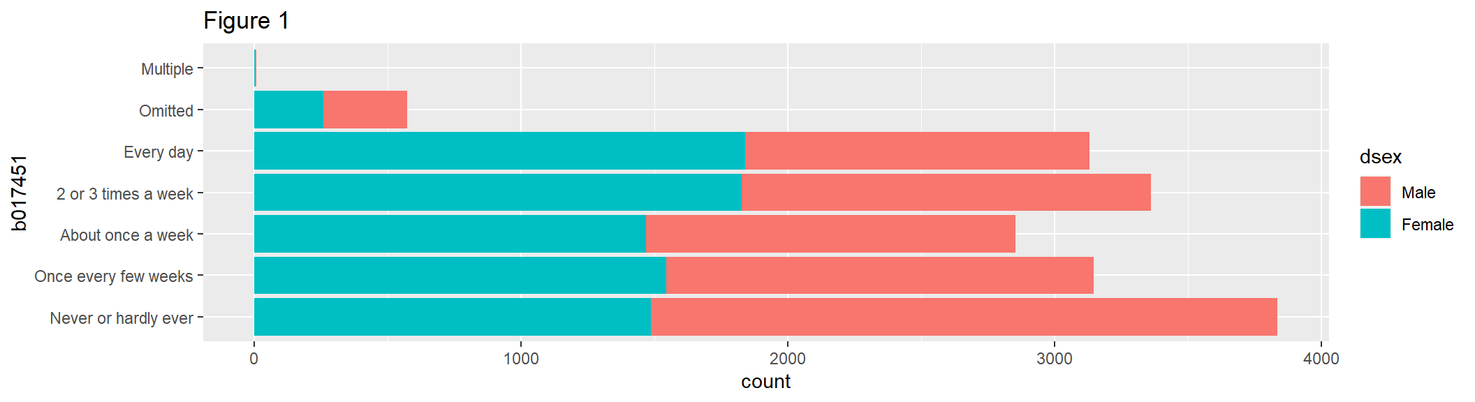
geom_histogram() uses binning to visualize the distribution of continuous variables. Figure 2 is a basic histogram that uses the first plausible value of the composite, giving an unbiased (but unweighted) estimate of the frequencies in each bin.
hist1 <- ggplot(gddat, aes(x = mrpcm1)) +
    geom_histogram() +
    labs(title = "Figure 2")
hist1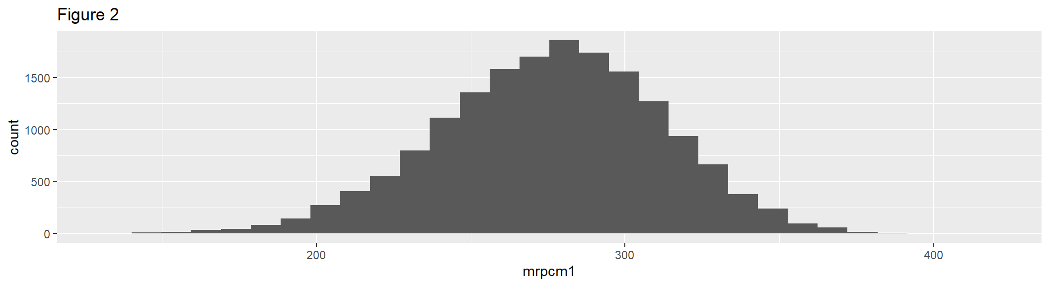
Figure 3 extends Figure 2, faceted on the categorical variable dsex, so that the output will be two histograms with common axes.
hist2 <- ggplot(gddat, aes(x = mrpcm1)) +
  geom_histogram(color = "black", fill = "white")+
  facet_grid(dsex ~ .) +
  labs(title = "Figure 3")
hist2
#> Warning: Combining variables of class <lfactor> and <factor> was
#> deprecated in ggplot2 3.4.0.
#> ℹ Please ensure your variables are compatible before
#>   plotting (location: `join_keys()`)
#> This warning is displayed once every 8 hours.
#> Call `lifecycle::last_lifecycle_warnings()` to see where
#> this warning was generated.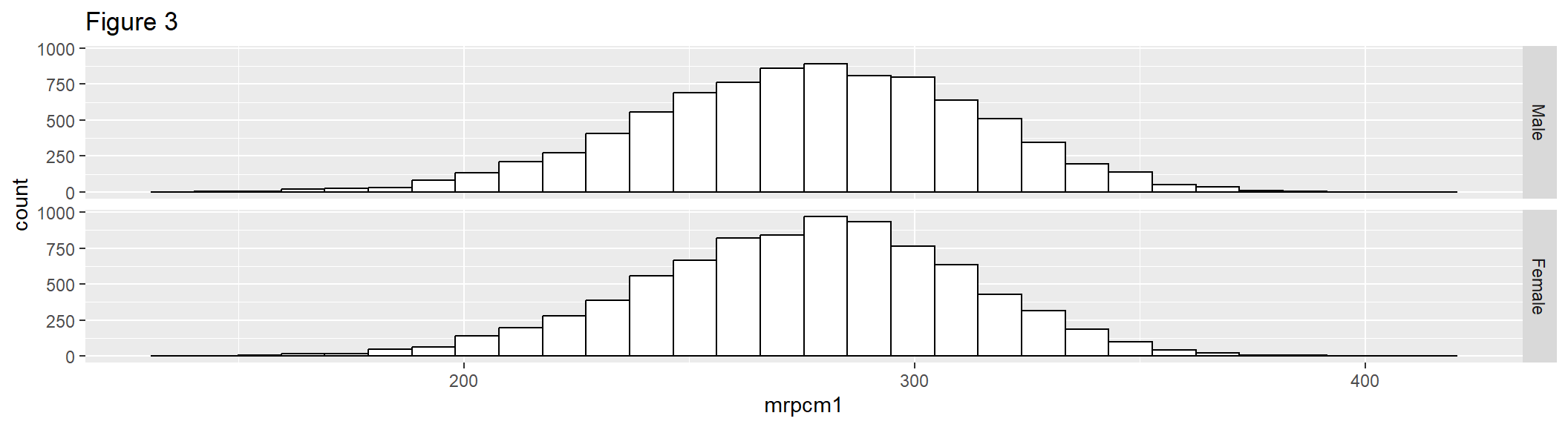
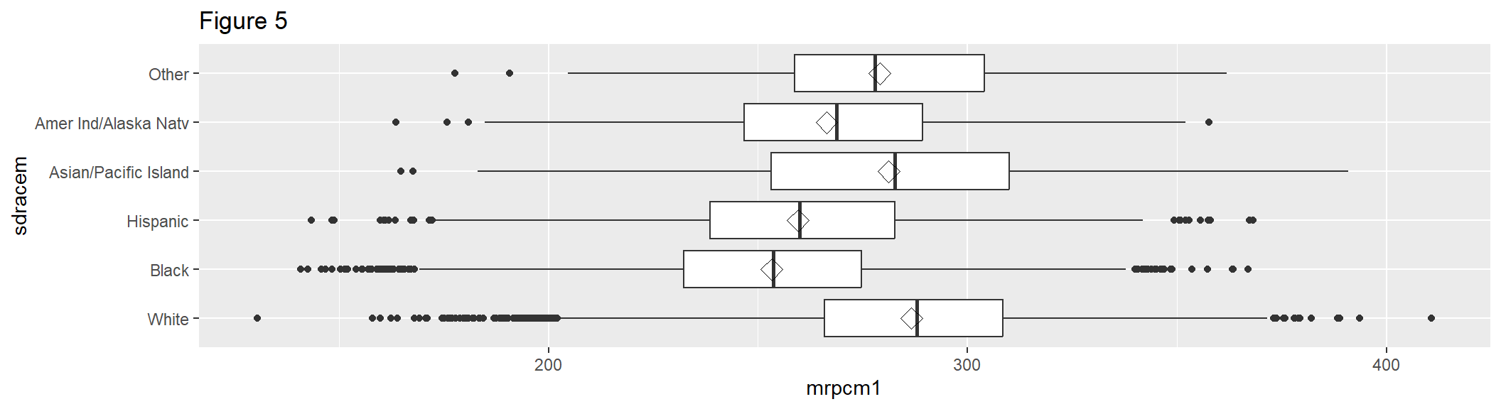
geom_boxplot() shows the distribution of a single variable through quartiles. Figure 4 shows the distribution of the six levels of the sdracem variable by the first plausible value of the composite.
box1 <- ggplot(gddat, aes(x = sdracem, y = mrpcm1)) +
  geom_boxplot() +
  labs(title = "Figure 4")
box1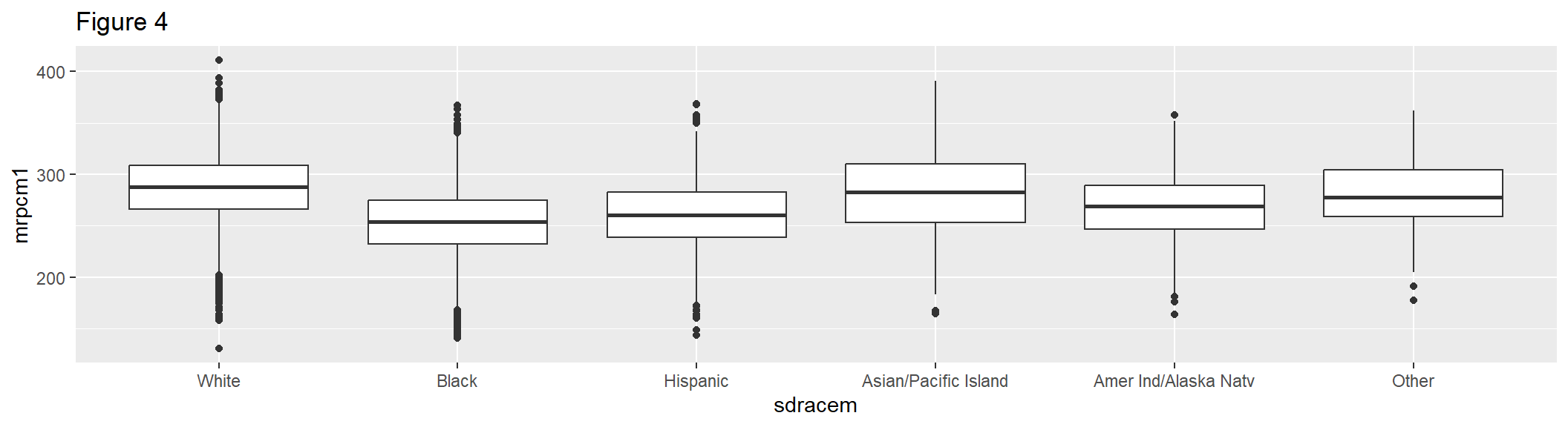
Figure 5 extends Figure 4 by using stat_summary() to add another statistic on top: the mean of mrpcm1 by sdracem, which is represented by the diamond-shaped symbol (shape = 23). Figure 5 also adds a coordinate flip via coord_flip().
box2 <- box1 + stat_summary(fun.y = mean, geom = "point", shape = 23, size = 4) +
  coord_flip() +
  labs(title = "Figure 5")
box2